ProjectSelf-study · Python · Simulation

Classical mechanics simulator

An interactive, extensible library of physics simulations built from a self-taught MIT 8.01 classical-mechanics course: each one a small differential equation you can poke, plot and play with.

TypePersonal project (self-study)

LanguagePython

StackNumPy · Dear PyGui

TopicClassical mechanics (MIT 8.01)

Git repo

Overview

This is a desktop application built alongside MIT OpenCourseWare's 8.01 Classical Mechanics^[1]: a small physics engine paired with a growing library of interactive simulations. Each topic from the course (projectile motion, friction on an incline, oscillations, gravitation, chaos) becomes a tweakable, plottable toy. As much as it is about the physics, it is an exercise in clean, extensible software architecture, which is most of what this writeup covers.

From coursework to sandbox

The course is self-taught, and worked problems on paper only go so far. The idea was to make each concept interactive: launch a projectile and add air drag, detune a driven oscillator until it beats, or nudge a double pendulum into chaos, then watch the equations actually play out.

One sandbox, not a pile of scripts

Rather than write a throwaway script per topic, I wanted a single sandbox where every simulation shares the same machinery: parameters I can drag, presets that jump between regimes, live plots, and the governing equations drawn on screen. That decision is what turned a study aid into a small but genuinely extensible piece of software.

Architecture: three clean layers

The project is split into three layers that know almost nothing about each other: a physics core, a library of simulations, and a UI shell. The core has no knowledge of any specific simulation; a simulation has no knowledge of the UI; the UI talks to a simulation through a tiny interface. Adding a new topic from the course is a matter of writing one file.

Everything is a first-order ODE

The unifying idea is that every simulation is a system of first-order ordinary differential equations. A simulation owns a state vector (positions and velocities, or angles and angular velocities, stored as a NumPy^[2] array) and implements one method, derivatives(state, t), returning the time derivative of that state. The core integrates it forward; the simulation itself never deals with a time step.

class Simulation(ABC):
    @abstractmethod
    def derivatives(self, state, t):   # returns d(state)/dt
        ...

# Two-body gravity. state = [x1, y1, x2, y2, vx1, vy1, vx2, vy2]
def derivatives(self, state, t):
    x1, y1, x2, y2, vx1, vy1, vx2, vy2 = state
    dx, dy = x2 - x1, y2 - y1
    r = sqrt(dx*dx + dy*dy + softening*softening)
    a = G / (r*r*r)
    return np.array([vx1, vy1, vx2, vy2,
                      a*m2*dx,  a*m2*dy,
                     -a*m1*dx, -a*m1*dy])

Every simulation reduces to one method: the time derivative of its state vector.

Pluggable numerical integrators

Because a simulation only ever says 'here is my derivative', the method used to step it forward in time is completely interchangeable. The core ships two, selected from a small registry and switchable live from the toolbar: a first-order Euler^[3] method and the classic fourth-order Runge-Kutta (RK4)^[4].

def rk4(state, t, dt, f):
    k1 = f(state,           t)
    k2 = f(state + k1*dt/2, t + dt/2)
    k3 = f(state + k2*dt/2, t + dt/2)
    k4 = f(state + k3*dt,   t + dt)
    return state + (k1 + 2*k2 + 2*k3 + k4) * (dt / 6)

The fourth-order Runge-Kutta step, one of two interchangeable solvers.

Making numerical error visible

Switch an orbit or a pendulum from RK4 to Euler, watch the energy plot, and the error becomes physical: the orbit slowly spirals outward and the pendulum gains amplitude from nowhere, because Euler quietly injects energy every step. RK4 keeps the same quantities visibly flat. It turns numerical integration error into something you can see rather than derive.

A library of classical mechanics

Six simulations cover the backbone of the course: projectile motion with optional quadratic drag and adjustable gravity; a block on an inclined plane with separate static and kinetic friction; a simple pendulum spanning the small-angle and fully nonlinear regimes; a spring-mass oscillator; a chaotic double pendulum^[5]; and a two-body gravitational orbit. The orbit's close-approach singularity is tamed with Plummer softening^[6].

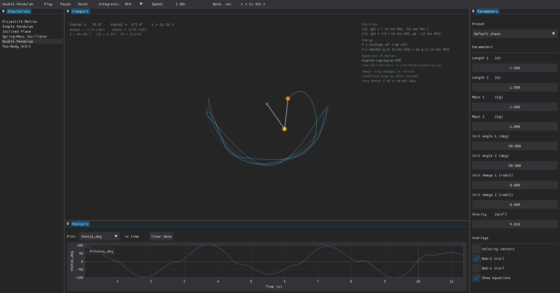
The simulator running the double pendulum, showing its traced path, an overlay of the equations of motion, a generated parameter panel and a plot of θ₁ against time — The chaotic double pendulum: the simulation library on the left, live state and equations overlaid on the viewport, the generated parameter panel on the right, and θ₁ plotted against time below.

Damped and driven oscillations

The spring-mass oscillator shows how much a single simulation can teach. Its presets walk through under-, critically- and over-damped motion, then add a sinusoidal drive to demonstrate resonance and beats. It obeys the damped, driven harmonic-oscillator equation:

m\ddot{x} + c\dot{x} + k x = F_0 \cos(\omega t)

The damped, driven harmonic oscillator behind the spring-mass simulation.

Conservation laws you can watch

Wherever a quantity should be conserved, the simulation records it so I can plot it. The orbit reports total energy and angular momentum under Newton's law of gravitation; the double pendulum tracks kinetic, potential and total energy. Watching those lines stay flat, or drift under a crude integrator, is the whole point.

F = \dfrac{G\,m_1 m_2}{r^{2}}

Newtonian gravitation, the force law driving the orbit simulation.

Self-describing simulations and the UI

Each simulation declares its parameters as plain data (a label, a range and a step), and the interface builds the controls from that declaration. The same holds for presets (named snapshots of initial conditions) and overlays (toggles for velocity arrows, force vectors, trails and the on-screen equations). Write a new simulation and it arrives with a full control panel, a plot selector and overlays, for free.

The application shell

The front end is a docking desktop app built with Dear PyGui^[7]: a library panel to pick a simulation, a viewport with a pan-and-zoom camera, the auto-generated parameter panel, and an analysis panel that plots any recorded variable against time. A toolbar handles play, pause and reset, the live integrator switch and a simulation-speed multiplier, and the window layout persists between runs. The main loop is real-time, advancing each simulation by the frame's elapsed time, clamped and then scaled by the speed control.

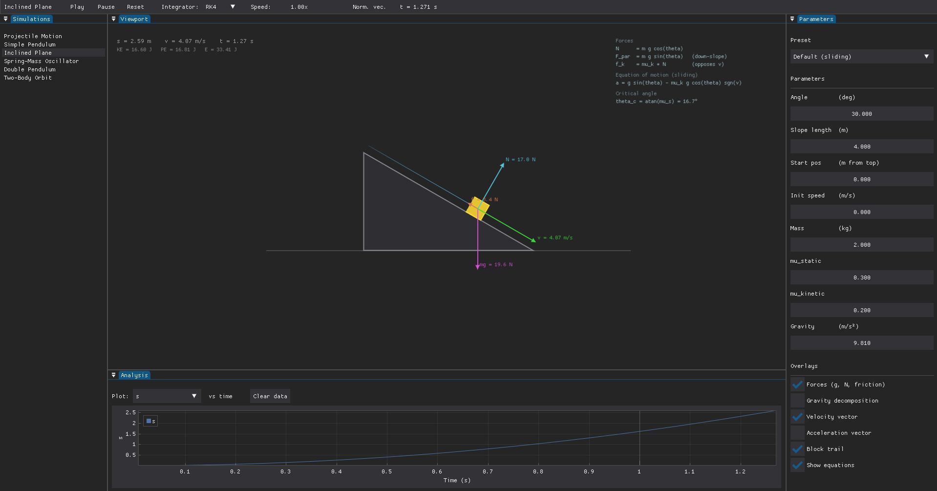
The simulator running a block sliding down a 30-degree incline with weight, normal and velocity vectors drawn, next to its parameter panel and a distance-against-time plot — The inclined-plane simulation with the force and equation overlays enabled. Every control on the right (preset, parameters and overlay toggles) is built from the simulation’s own declaration.

Packaging and takeaways

The app bundles into a standalone Windows executable with PyInstaller^[8], so it runs without a Python install. The project made a few things concrete that the coursework alone could not: numerical integration stopped being a formula and became something with visible, debuggable error; conservation laws turned into lines you can watch hold or fail; and the clean core, library and UI split meant each new concept became a new simulation in minutes rather than a new program.

References

Back to projects Marching Cubes & procedural worlds